Unconstrained Optimization in .NET (C# and Visual Basic)
This section describes the options for finding minima of nonlinear scalar functions $f(x)$ in ILNumerics Ultimate VS Optimization Toolbox:
; where
Note that the term 'scalar function' refers to the dimensionality of the function output only. A scalar function accepts n input parameters but generates only a single output parameter. So, the goal obviously is to find a vector $x$ of input parameters which minimizes the output of the function.
No restrictions are imposed on the vector $x$ whatsoever. Therefore, we are dealing with unconstrained optimization problems here: any $x \in \mathbb{R}^n$ is allowed which minimizes the objective function $f$. However, in general special floating point values as double.PositiveInfinity and double.NaN are not allowed.
Three algorithms are available for these kind of minimization problems. They differ in the method used to compute the hessian matrix of $f$ which greatly influences the performance but also the precision of the algorithms.
Common API for unconstrained optimization
The common entry point fmin() can be used for simple optimization problems:
- Optimization.fmin - common API function for scalar problems.
fmin is able to handle unconstrained and constrained problems. Unconstrained problems are solved by ommiting any constraint parameters from the fmin parameter list. Consult the constrained optimization documentation in order to lear more about Optimization.fmin.
Specialized API for unconstrained optimization
A list of specialized API functions exist for direct access to the unconstrained minimization methods. Choosing an unconstrained method explicitly is recommended in situations where a better performance or more control over the optimization run is needed:
- Optimization.fminunconst_newton is a newton method solver. The hessian matrix is evaluated explicitely in each iteration step. Custom hessian functions can be provided. This method brings good results for small and mid-scale problems. However, the explicit evaluation of the hessian is costly for larger problems.
- Optimization.fminunconst_bfgs is a quasi newton method which prevents the explicit evaluation of the true hessian matrix by computing an estimate based on the BFGS algorithm. This is the recommended method in most situations.
- Optimization.fminunconst_lbfgs reduces the memory requirements of the BFGS solver by computing subsequent steps based on a reduced 2nd derivative as a replacement for the full hessian matrix. This method is recommended for large scale problems.
We will describe these methods in the subsequent paragraphs.
Usage of unconstrained optimization
All methods for unconstrained optimization share the same name prefix Optimization.fminunconst_??? and have a similar interface:
All methods expect
- a delegate for the objective function,
- an initial guess for the solution,
- a number of optional parameters, controlling the iterations and exit conditions, and
- a number of optional output parameters, gathering further details from the computation.
In the remaining paragraphs of this section we explain the usage of those parameters. This will be valid for all of the functions similarly. However, we will only take the BFGS variant as an example if not otherwise stated.
Obligatory Parameters
Objective functions in ILNumerics.Optimization are defined as ILNumerics.Optimization.ObjectiveFunction<T> delegates: expecting a single vector shaped array X with the position of the current iteration and returning a scalar. Currently, all unconstrained (and also all constrained) solvers are able to deal with functions working on double precision values only: ObjectiveFunction<double>.
Example of an objective function for $$f(x) = x_1^2 + x_2^2 + 2$$
The objective function gets called potentially a large number of times during the optimization algorithm, probing the current intermediate solution at each iteration step down to the minimum. Therefore, its implementation should be as simple and fast as possible. Prevent from extensive error checks in your objective function! The input arguments are provided by the algorithm automatically, so checks for the size, shape and state of input parameters are commonly not needed. Read down for multiple options of dealing with performance issues.
An initial guess is provided to the optimization function:
The following image shows a plot of this function. A red dot marks the minimizer M as found by the BFGS algorithm. The full example is found in the examples section.
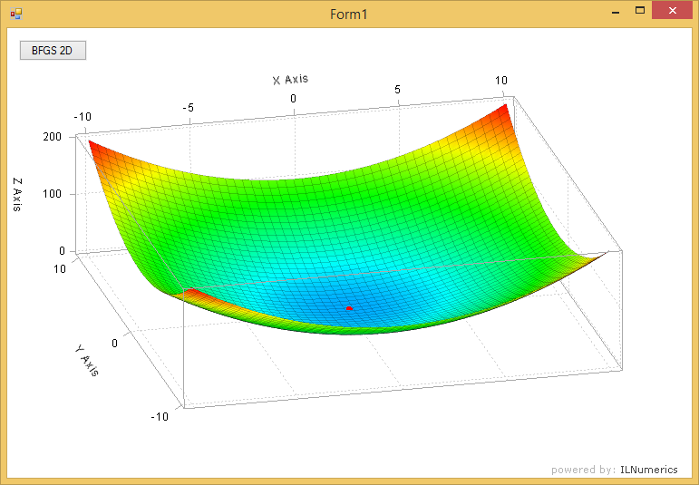
The initial guess is obligatory because all optimization methods target local minima only. For convex functions like the one in the example above the single minimum is identical with the global minimum. However, since arbitrary, non-convex functions have multiple minima the initial guess provided by the user will determine which extrema we are interested in.
The initial guess should be as close to the expected minima as possible. This will not only speed up the algorithm, since fewer steps are required for finding the optimal result. It will also ensure that the intended minima is found for non-convex functions like the following:
The return value of any Optimization.fminunconst_???() function corresponds to the local minimizer of the function, i.e. the vector $\tilde{x}$ which minimizes the objective function. All small changes of $\tilde{x}$ will lead to larger values of the objective function. Or, mathematically spoken: $$f(\tilde{x}^*) > f(\tilde{x}) \;for \;\tilde{x} \in N(\tilde{x}^*)$$
where $N(\tilde{x}^*)$ is a neighborhood of $\tilde{x}$. The convex example above reaches its minimum at the minimizer $(0,0)$, the minimum value is computed by evaluating the objective function at the minimizer, which gives $2$.
Providing optional Derivatives
By default, Optimization.fminunconst_????() determine the intermediate search steps to the final solution automatically. This is done by iteratively computing direction and width for subsequent steps from estimates of the first and second order derivatives of the objective function. Multiple evaluations of the objective functions at different points are necessary - just to get an estimate of the derivatives.
It is well known that the better the derivative estimates match the exact slope of the objective function the better the algorithm is able to find the minimum and the more exact the solution will be.
By default, ILNumerics.Optimization.fminunconst_bfgs() automatically computes the gradient (first derivative of $f$) by an approach based on finite differences:
- ILNumerics.Optimization.jacobian_prec - precise estimate of the derivative. This function uses a forward and backward finite differences approach with automatic step size tuning and Ridders' method of polynomial extrapolation. This will give very accurate results and usually leads to much fewer steps to the final solution. However, computing accurate estimates is rather expensive and potentially lead to poor performance. jacobian_prec is the default.
- ILNumerics.Optimization.jacobian_fast - estimation of the derivatives with orientation towards speed rather than accuracy. This function uses a forward finite differences approach, a simple stepsize computation (with a fallback to the more advanced algorithm used in jacobian_prec). This leads to fewer evaluations of the objective function to the cost of less accurate results. One may notice a great speed-up in comparison to jacobian_prec for large scale functions. However, the reduced accuracy may or may not lead to more iteration steps to the final solution. This function is recommended for "good behaving" objective functions.
Default Derivative Function
It is possible to chose which function is used for the computation of a derivative. Users can specify the function either
- locally - for the current optimization run, by providing a derivative function as the gradientFunc parameter, or
- globally - for all subsequent optimization runs, by configuring the static DefaultDerivativeFunction member of the ILNumerics.Optimization class.
After ILNumerics was started, the DefaultDerivativeFunction is set to jacobian_prec. One can modify the default function used by all optimization methods, by redirecting the DefaultDerivativeFunction to some other function:
If no gradientFunc parameter was provided the function pointed to by DefaultDerivativeFunction is used. If the gradientFunc parameter does point to a derivative function, this one is used instead of the default derivative function.
Custom Gradient Functions
ILNumerics.Optimization offers the option to implement custom derivative functions. Users are enabled and encouraged to provide the exact derivative implementation (if known and efficiently implemented) or a custom, hand tuned estimation algorithm for the gradient.
All derivative functions have the same signature:
Next to the current position $x$, the objective function $func$ and the evaluation of the objective function $fx$ is provided. It is up to you, which one of the provided parameters to use. Choose those parameters, which are helpful for your implementation. If an analytical gradient definition is known, neither $func$ nor $fx$ are needed.
The gradient is defined as the vector of partial derivatives for each input dimension:$$\operatorname{grad}(f) = \frac{\partial f}{\partial x_{1}}\hat{e}_{1}+\cdots+\frac{\partial f}{\partial x_{n}}\hat{e}_{n}=\begin{pmatrix}\frac{\partial f}{\partial x_{1}}\\ \vdots\\ \frac{\partial f}{\partial x_{n}} \end{pmatrix}$$
Referring back to our first example of an objective function $$f(x) = x_1^2 + x_2^2 + 2$$ the gradient turns out to be $$\operatorname{grad}(f) = \begin{pmatrix}2x_1\\2x_2\end{pmatrix}$$
A custom implementation, therefore would simply give:
Note, how the gradient is provided as row vector here! The reason lays in the fact that the DerivativeFunction<T> delegate is generalized to vector sized functions $f$. This enables it to be used for other optimization methods, dealing with vector sized objective functions, namely nonlinear least mean squares optimization. Here, the first derivative builds up the jacobian matrix with the transposed gradients of the function components as rows. Returning the gradient as row vector nicely corresponds to the special case of a scalar function.
A Note on Performance
Specifying an exact gradient is recommended and usually pays off in terms of performance and precision of the result. However, in many situations and if no analytical function is known, custom gradient estimation functions can still improve the optimization process. When using such a custom gradient estimation function, one usually relies on the frequent evaluation of the objective function. In order to minimize these evaluations (they are commonly the major bottleneck in an optimization run), the API of Optimization.DerivativeFunction<T> provides the fx parameter. If during the algorithm the objective function has been evaluated at the current position x already, the result is provided in fx.
However, one should not rely on fx being provided always! Rather use a scheme which first tests on fx being not null and evaluates the objective function only if fx was found to be null:
Custom Hessian Implementation
The main difference between all unconstrained solvers in ILNumerics.Optimization is how they deal with the second derivative of the objective function. While BFGS and L-BFGS create useful replacements for the full hessian matrix, the fminunconst_newton method evaluates the hessian in each iteration step.
What is true for the gradient computation holds for the hessian computation: One can improve performance, robustness and precision of the iterative process by providing a custom hessian function. If an exact analytical expression of the 2nd derivative of the objective function is known and if an efficient implementation exists, providing a custom hessian implementation can drastically decrease the iteration steps needed for the fminunconst_newton method.
Just like for gradient /jacobian functions, the hessianfunc parameter of fminunconst_newton accepts a function as Optimization.DerivativeFunction<T> delegate. Note that both, fminunconst_bfgs and fminunconst_lbfgs do not accept custom hessian functions.
Controlling the Optimization Process
The progress of the optimization can be further controlled by various parameters. One can limit the number of overall iterations and the exit conditions. These parameters can be used to control the maximum time spent in the minimization loop and the precision of the solution. This can be generally useful for 'bad behaving' functions, like those with very flat slopes. An example is provided below.
Iteration Count
The optional maxIter parameter is used to limit the overall iteration count. Common values range from 50 to 2000. The best value depends on the objective function and the derivatives provided. Commonly, BFGS algorithms on simple functions converge in much less iterations. If the algorithm hits the limit, this is usually a good indication of a problematic objective function or an erroneous derivative implementation or a too low error tolerance value requested. The default value for maxIter is 500.
Exit Conditions
tol is an optional parameter specifying the quality of the gradient requested before exiting the iteration loop. By quality we mean the improvement of the gradient compared to the gradient at the starting position $x_0$. Since at the exact solution $x_{opt}$ the gradient $\operatorname{grad}(f(x_{opt})) = \vec0$ is expected to be $\vec0$, tol gives the factor by which the initial gradient must be decreased in order to be considered 'good enough'. The decision is based on the infinity norm $$\Big|\operatorname{grad}(f)\Big|_{\infty}$$
The default tolerance is $1e^{-8}$.
tolX controls another way out of the minimization iterations, based on the displacement of the current iteration solution $x$. Once the algorithm stops making significant progress and the solution vector is not changing significantly, we consider the current solution as 'good enough'. tolX gives the minimal distance subsequent iterations must improve on the solution vector in order to keep searching for better solutions. Note that for large $x$ smaller steps as given by tolX may be accepted in order to increase robustness of the algorithm.
One can tune the default values for tol and tolX by help of the static property Optimization.DefaultTolerance.
Gathering Progress Information
Users can query a collection of additional details about the minimization process after it was finished.
Information include the number of iterations needed, the norm of the gradient $||\operatorname{grad}(f(\tilde{x}))||^2$ after each iteration step, and the intermediate solution vectors $\tilde{x}$. These options are demonstrated in the following on a more difficult objective function: the Rosenbrock function[1] $$f(\mathbf{x}) = \sum_{i=1}^{N-1} \left[(1-x_i)^2+ 100 (x_{i+1} - x_i^2 )^2 \right] \quad \forall x\in\mathbb{R}^N.$$
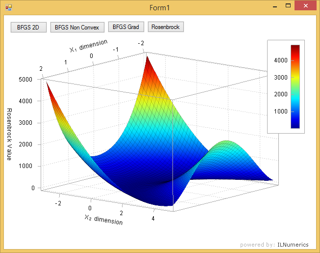
The n-dimensional Rosenbrock function is implemented in ILNumerics Optimization Toolbox among other test functions. The minimum of the 2D variant is known to be found at [1,1]. In order to get the number of iterations needed by BFGS and L-BFGS to obtain the minimum of the 2D Rosenbrock function, we do:
Both functions found a minimizer at [1,1]. fminunconst_bfgs managed to find the solution in much less iterations compared to L-BFGS. Also, the solution is much more accurate. While most optimizer implementations are able to find the minimum of the rosenbrock function up to a precision of 1e-6 only, fminunconst_bfgs gets as close as 7 * 10-13! One reason for this is due to its very accurate derivative computation and sophisticated line search implementation.
Following the Iteration Steps
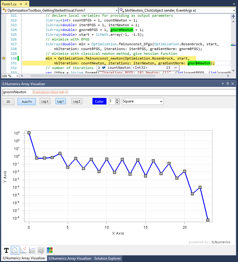
In order to get details about the path to the final solution for an optimization run, we can utilize the iterations and gradientNorm parameters of the fminunconst_??? methods. Both are optional output parameters and are applied as follows:
Both, iterations and gradientNorm parameters can be used to visualize the progress of the algorithm and to value the iteration path and the result. In the following image the intermediate steps found by BFGS and Newton are plotted on top of the objective function (Rosenbrock function). The norm of the gradient is plotted as a logarithmic line plot for both algorithms. The vaues returned by gradientNorm are a valuable indicator for the quality of the results. Usually, for a straight path to the minimum, intermediate steps should show decreased $norm(grad(f(x)))$ values. At the minimizer $x^*$, the gradient optimally gets close to $\vec0$:
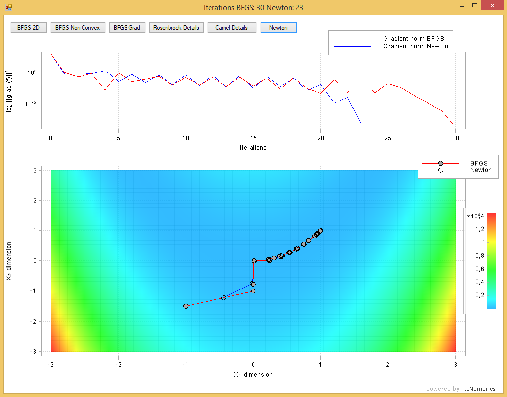
Those visualizations often help to decide for the best algorithm fit and to tune the input parameters for the optimizations. From the above image it gets clear that the Newton method took the straightest path to the solution while BFGS used 7 steps more to get to the same minimum.
In general the Array Visualizer comes in handy to visualize both parameters right within your debug session:
Download the complete runnable example from the examples section.
Technical Notes
The BFGS algorithm implemented in ILNumerics is a Quasi-Newton algorithm based on iterative update steps using a Gauss Conjugate Gradient and a line-search algorithm based on the Golden Section Search to solve the Wolfe-Powell’s conditions. The Newton variant (by default) computes the hessian matrix based on a forward-backward finite differences algorithm with Ridders' method of polynomial extrapolation. L-BFGS uses a trust-region method for finding new update steps.
Robustness: Even in the range of “big" numbers, the algorithms will manage to adapt. However, it is recommend to normalize / scale the objective functions provided to reach a good floating point precision range (i.e.: values ‘near' 1.0).
Memory needs: The quasi-Newton BFGS method and the Newton method have $O(n^2)$ memory requirement, where the L-BFGS has $O(n)$ memory requirement. Therefore, the BFGS algorithm and the classical adaptive Newton method are available for small and medium sized unconstrained optimization problems. The L-BFGS is preferred for large scale optimization problems.
References
See: The generalized Rosenbrock's function (http://www.it.lut.fi/ip/evo/functions/node5.html)