ILNumerics for Science – How did you do the Visualization?

In the third part of our series we focus on the visualization of scientific data. You learn how to easily display your data with ILNumerics and the ILPanels.

Reactions

I got a lot of emails after the last two posts (first, second) of people that liked the post and are interested in learning more. Most emails asked me to go into more details about how I did all that. Obviously, not too many people are interested in implementing the particle in a box, so the “what” is not as interesting as the “how”.

In this post I want to focus on the visualization part of the previous two examples and how ILNumerics helped me. As many of our users are scientists and engineers they are typically experts in the computation part but appreciate a little help in the visualization. If you’re interested in the computation part, please be patient until the next post.

The Form

I started by creating a new project in Visual Studio and chose Windows Forms Application. This gives me a vanilla Form1.cs. That’s the basis of all the visualization and helps me – being a scientist and not a coder – a lot, because I couldn’t do all that without the help of Visual Studio in the background.

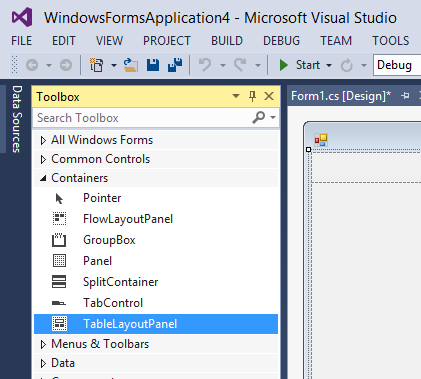
On the left-hand side in the Toolbox panel I picked TableLayoutPanel under Containers and dragged it into Form1.cs.

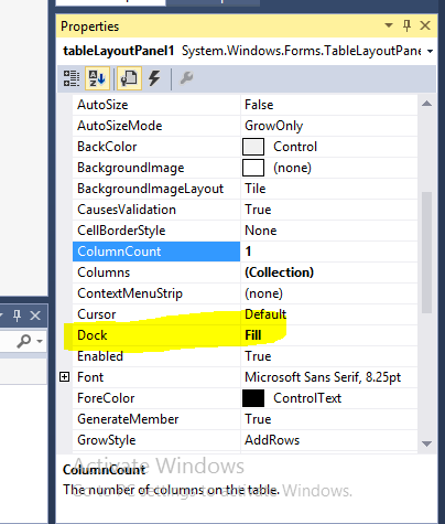
I adjusted the table to have three rows and a single column. In the Properties section under Dock I chose Fill so that everything scales when scaling the window later on.

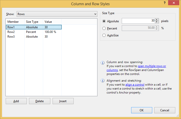
A right click on Table -> Edit Rows and Columns allows you to change the behavior of the three rows. I wanted the first and last row not to scale when changing the window. This is what I chose here.

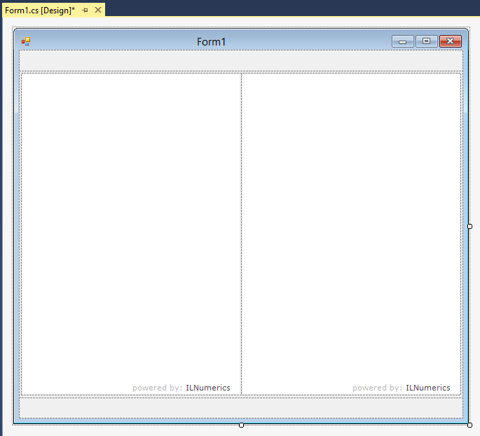
In the middle row we would like to see two ILNumerics panels. So I dragged another TableLayoutPanel in the middle row and chose two columns and one row. Choosing Dock = Fill for the new table and dragging two ILPanels into the respective columns (again with Dock = Fill) gives us the layout for our final Windows Form.

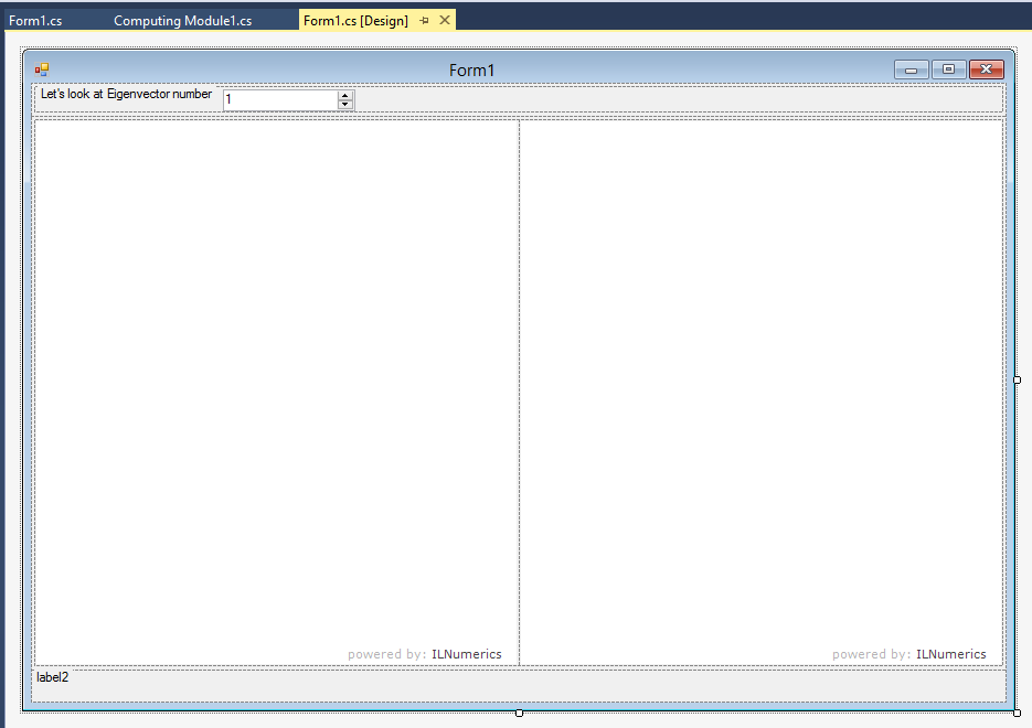
In the header (the first row) I inserted a FlowLayoutPanel that makes sure that everything in there will be displayed rather neatly. Then I added the labels and the NumericUpDown according to my needs. Please make sure that you go through the properties of every item and choose the values according to your needs. In my case, for instance, the minimum value for the state is 1, since 0 would mean that there is no particle present. Here is the final picture of the form for the 1D particle in a box:

The Wiring

After having the layout ready the interactivity needs to be implemented. In this case there is only one point of user interaction. The user can choose which eigenvector to display. Double-clicking on the NumericUpDown control opens a new tab with a predefined class and a function handling the event when a user changes the value of the eigenvector.

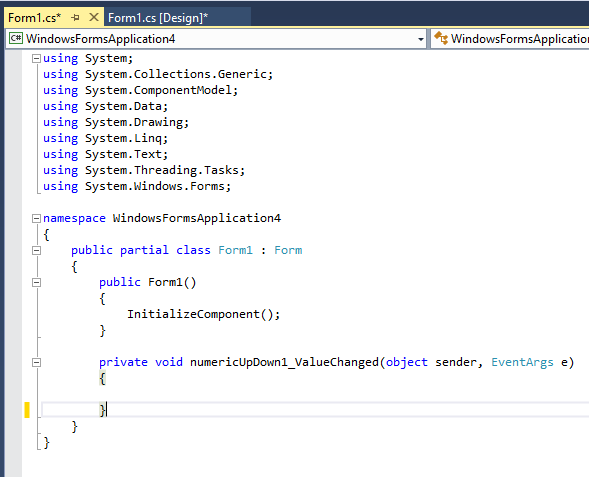
All that’s needed now is to implement the function numericUpDown1_ValueChanged. This is particularly simple in our case. We just call the Update function (still to be implemented) with the new value for the eigenvector.

In the case of the 2D particle in a box we have, in fact, four events that should trigger the Update function. This is easily done by introducing these lines of code in the public function Form1():

     numericUpDown1.ValueChanged += Update;
     numericUpDown2.ValueChanged += Update;
     numericUpDown3.ValueChanged += Update;
     textBox1.TextChanged += Update;

The Implementation

Now, all we need to do is to implement the Update function and the initialization. The initialization makes sure that all the plotting objects are created when starting the program.

     public Form1()
     {
        InitializeComponent();

        var EVID = 1;
        var MeshSize = 1000;

        InitializePanel1(EVID, MeshSize);
        InitializePanel2(EVID, MeshSize);

        label2.Text = string.Format("In appropriate units the energy is {0}", EVID * EVID);
     }

     private void InitializePanel1(int EVID, int MeshSize)
     {
        ILArray<float> XY = ILMath.tosingle(Computing_Module1.CalcWF(EVID, MeshSize));
        var color = Color.Black;
        ilPanel1.Scene =
          new ILScene {
            new ILPlotCube {
              new ILLinePlot (XY, lineColor : color)
            }
          };
     }

The call to Computing_Module1.CalcWF will be explained in the next post. The piece of code above initializes the wave function plot and the density plot in their respective panels with the first eigenvector and a mesh size of 1000.

Finally, the Update function is implemented.

     private void Update(int EVID, int MeshSize = 1000)
     {
       ILArray<float> XY = ILMath.tosingle(Computing_Module1.CalcWF(EVID, MeshSize));
       ilPanel1.Scene.First<ILLinePlot>().Update(XY);
       ilPanel1.Scene.First<ILPlotCube>().Reset();
       ilPanel1.Refresh();

       ILArray<float> XD = ILMath.tosingle(Computing_Module1.CalcDensity(EVID, MeshSize));
       ilPanel2.Scene.First<ILLinePlot>().Update(XD);
       ilPanel2.Scene.First<ILPlotCube>().Reset();
       ilPanel2.Refresh();
       label2.Text = string.Format("In appropriate units the energy is {0}", EVID * EVID);
     }

Again, the CalcWF and CalcDensity calls will be explained in the next post. The Reset() function rescales the axes and the Refresh() function finally puts the new plot on screen.