Tag Archives: computing

N-dim Array Broadcasting Efficiency in ILNumerics 4.10

Next to other great improvements in version 4.10 of ILNumerics Ultimate VS, it is especially one new feature which requires some attention: general broadcasting for n-dimensional ILArrays.

Broadcasting as a concept today is found in many popular mathematical prototyping systems. The most direct correspondence probably exists in the numpy package. Matlab and Octave offer similar functionality by means of the bsxfun function.

The term ‘broadcasting’ refers to a binary operator which is able to apply an elementwise operation to the elements of two n-dimensional arrays. The ‘operation’ is often as simple as a straight addition (ILMath.add, ILMath.divide, a.s.o.). However, what is special about broadcasting is that it allows the operation even for the case where both arrays involved do not have the same number of elements.

Broadcasting in ILNumerics prior Version 4.10

In ILNumerics, broadcasting is available for long already. But prior version 4.10 it was limited to scalars operating on n-dim arrays and vectors operating on matrices. Therefore, we had used the term ‘vector expansion’ instead of broadcasting. Obviously, broadcasting can be seen as a generalization of vector expansion.

Let’s visualize the concept by considering the following matrix A:

A

1  5   9  13  17
2  6  10  14  18
3  7  11  15  19
4  8  12  16  20

Matrix A might represent 5 data points of a 4 dimensional dataset as columns. One common requirement is to apply a certain operation to all datapoints in a similar way. In order to, let’s say, scale/weight the components of each dimension by a certain factor, one would multiply each datapoint with a vector of length 4.


ILArray<double> V = new[] { 0.5, 3.0, 0.5, 1.0 };

0.5
3.0
0.5
1.0

The traditional way of implementing this operation would be to expand the scaling vector by replicating it from a single column to a matrix matching the size of A.

VExp = repmat(V, 1, 5); 

0.5  0.5  0.5  0.5  0.5
3.0  3.0  3.0  3.0  3.0
0.5  0.5  0.5  0.5  0.5
1.0  1.0  1.0  1.0  1.0

Afterwards, the result can be operated with A elementwise in the common way.

ILArray<double> Result = VExp * A;

0.5   2.5   4.5   6.5   8.5
6.0  18.0  30.0  42.0  54.0
1.5   3.5   5.5   7.5   9.5
4.0   8.0  12.0  16.0  20.0

The problem with the above approach is that the vector data need to be expanded first. There is little advantage in doing so: a lot of new memory is being used up in order to store completely redundant data. We all know that memory is the biggest bottleneck today. We should prevent from lots of memory allocations whenever possible. This is where vector expansion comes into play. In ILNumerics, for long, one can prevent from the additional replication step and operate the vector on the matrix directly. Internally, the operation is implemented in a very efficient way, without replicating any data, without allocating new memory.

ILArray<double> Result = V * A;

0.5   2.5   4.5   6.5   8.5
6.0  18.0  30.0  42.0  54.0
1.5   3.5   5.5   7.5   9.5
4.0   8.0  12.0  16.0  20.0

Generalizing for n-Dimensions

Representing data as matrices is very popular in scientific computing. However, if the data are stored into arrays of other shapes, having more than two dimensions, one had to fall back to repmatting in order for the binary operation to succeed. This nuissance has been removed in version 4.10.

Now it is possible to apply broadcasting to two arrays of any matching shape – without the need for using repmat. In order for two arrays to ‘match‘ in the binary operation, the following rules must be fullfilled:

  1. All corresponding dimensions of both arrays must match.
  2. In order for two  corresponding dimensions to match,
    • both dimensions must be of the same length, or
    • one of the dimensions must be of length 1.

An example of two matching arrays would be a vector running along the 3rd dimension and a 3 dimensional array:

3D Cubes 4 Broadcasting2
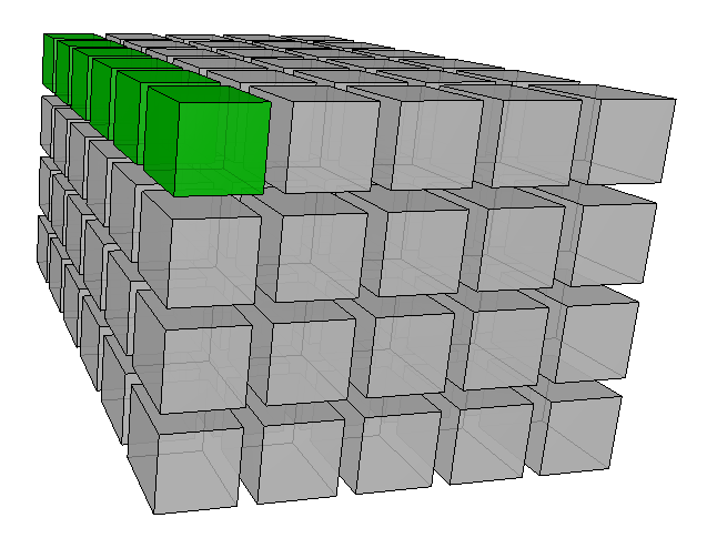
In the above image the vector (green) has the same length as the corresponding dimension of the 3D array (gray). The size of the vector is [1 x 1 x 6]. The size of the 3D array is [4 x 5 x 6]. Hence, any dimension of both, the vector and the 3D array ‘match’ in terms of broadcasting. A broadcasting operation for both, the vector and the array would give the same result as if the vector would be replicated along the 1st and the 2nd dimensions. The first element will serve all elements in the first 4 x 5 slice in the 1-2 plane. This slice is marked red in the next image: 3D Cubes 4 Broadcasting_slice
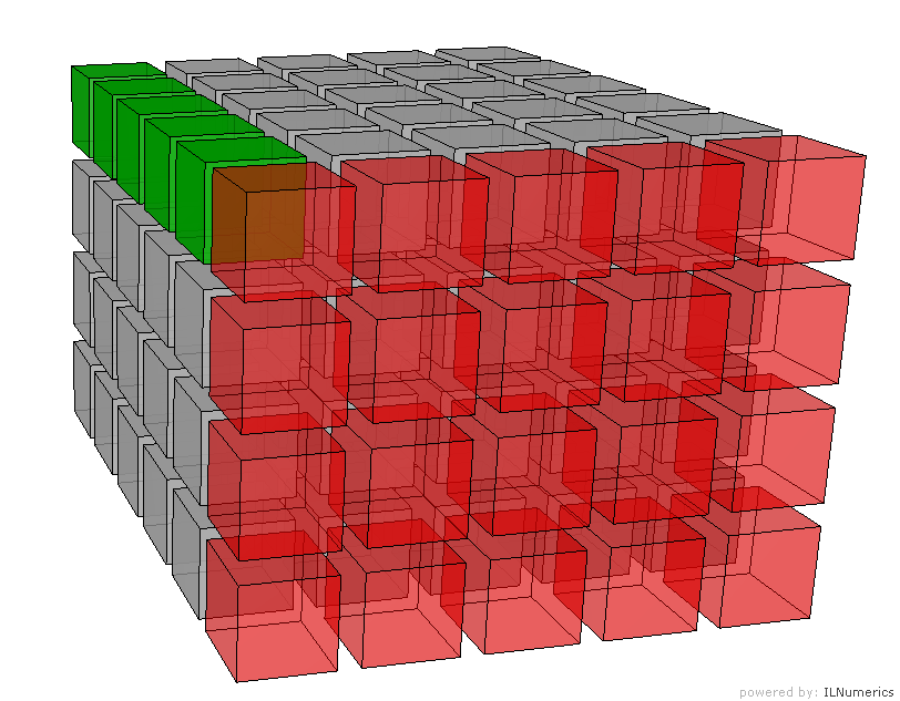
Note that all red elements here derive from the same value – from the first element of the green vector.  The same is true for all other vector elements: they fill corresponding slices on the 3D array along the 3rd dimension.

Slowly, a huge performance advantage of broadcasting becomes clear: the amount of memory saved explodes when more, longer dimensions are involved.

 Special Case: Broadcasting on Vectors

In the most general case and if broadcasting is blindly applied, the following special case potentially causes issues. Consider two vectors, one row vector and one column vector being provided as input parameters to a binary operation. In ILNumerics, every array carries at least two dimensions. A column vector of length 4 is considered an array of size [4 x 1]. A row vector of length 5 is considered an array of size [1 x 5]. In fact, any two vectors match according to the general  broadcasting rules.

As a consequence operating a row vector [1 x 5] with a column vector [4 x 1] results in a matrix [4 x 5]. The row vector is getting ‘replicated’ (again, without really executing the replication) four times along the 1st dimension, and the column vector 5 times along the rows.

array(new[] {1.0,2.0,3.0,4.0,5.0}, 1, 5) +array(new[] {1.0,2.0,3.0,4.0}, 4, 1)

<Double> [4,5]
[0]:          2          3          4          5          6
[1]:          3          4          5          6          7
[2]:          4          5          6          7          8
[3]:          5          6          7          8          9

Note, in order for the above code example to work, one needs to apply a certain switch:

Settings.BroadcastCompatibilityMode = false;

The reason is that in the traditional version of ILNumerics (just like in Matlab and Octave) the above code would simply not execute but throw an exception instead. Originally, binary operations on vectors would ignore the fact that vectors are matrices and only take the length of the vectors into account, operating on the corresponding elements if the length of both vectors do match. Now, in order to keep compatibility for existing applications, we kept the former behavior.

The new switch ‘Settings.BroadcastCompatibilityMode’ by default is set to ‘true’. This will cause the Computing Engine to throw an exception when two vectors of inequal length are provided to binary operators. Applying vectors of the same length (regardless of their orientation) will result in a vector of the same length.

If the ‘Settings.BroadcastCompatibilityMode’ switch is set to ‘false’ then general broadcasting is applied in all cases according to the above rules – even on vectors. For the earlier vector example this leads to the resulting matrix as shown above: operating a row on a column vector expands both vectors and gives a matrix of corresponding size.

Further reading: binary operators, online documentation

ILNumerics for Scientists – Going 3D

Recap

Last time I started with one of the easiest problems in quantum mechanics: the particle in a box. This time I’ll add 1 dimension and we’ll see a particle in a 2D box. To visualize its wave function and density we need 3D surface plots.

2D Box

This time we have a particle that is confined in a 2D box. The potential within the box is zero and outside the box infinity. Again the solution is well-known and can be found on Wikipedia. This time the state of the wave function is determined by two numbers. These are typically called quantum numbers and refer to the X and the Y direction, respectively.

The absolute size of the box doesn’t really matter and we didn’t worry about it in the 1D case. However, the relative size of the length and the width make a difference. The solution to our problem reads

$\Psi_{n,k}(x,y) = \sqrt{\frac{4}{L_x L_y}} \cdot \sin(n \cdot \pi \cdot x / L_x) \cdot \sin(k \cdot \pi \cdot y / L_y)$

The Math

Very similar to the 1D case I quickly coded the wave function and the density for further plotting. I had to make sure that the arrays are fit for 3D plotting, so the code looks a little bit different compared to last post’s

     public static ILArray<double> CalcWF(int EVXID, int EVYID, double LX, double LY, int MeshSize)
     {
        ILArray<double> X = linspace<double>(0, LX, MeshSize);
        ILArray<double> Y = linspace<double>(0, LY, MeshSize);

        ILArray<double> Y2d = 1;
        ILArray<double> X2d = meshgrid(X, Y, Y2d);

        ILArray<double> Z = sqrt(4.0 / LX / LY) * sin(EVXID * pi * X2d / LX) * sin(EVYID * pi * Y2d / LY);

        return Z.Concat(X2d,2).Concat(Y2d,2);
     }

Again, this took me like 10 minutes and I was done.

The Visualization

This time the user can choose the quantum numbers for X and Y direction, the ratio between the length and the width of the box and also the number of mesh points along each axis for plotting. This makes the visualization panel a little bit more involved. Nevertheless, it’s still rather simple and easy to use. This time it took me only 45 minutes – I guess I learned a lot from last time.

The result

Here is the result of my little program. You can click and play with it. If you’re interested, you can download the Particle2DBox source code. Have fun!

Particle2DBoxThis is a screenshot of the application. I chose the second quantum number along the x axis and the fourth quantum number along the y axis. The box is twice as long in y direction as it is in x direction. The mesh size is 100 in each direction. On the left hand side you see the wave function and on the right hand side the probability density.

ILNumerics for Scientists – An easy start

Motivation

I’ve been working as a scientist at universities for 10 years before deciding to go into industry. The one thing I hated most was coding. At the end of the day coding for scientists is like running for a football player. Obviously, you need it but it’s not what you’re here for.

I really dreaded the coding and the debugging. So much precious time for something that was so clear on paper and I just wanted the solution of my equations to see whether my idea made sense or not. More often than not scientists find that their idea was not so great and now they had spent so much time coding just to find out that the idea didn’t work. Continue reading ILNumerics for Scientists – An easy start

Scientific Computing Online: IPython Notebook, Shiny (R) and ILNumerics

It seems that we’re facing a trend at the moment: scientific computing, math and visualization software for web browsers. With our interactive web examples we have taken a step into that direction, too: Visitors of our website can change the C# code of our plotting and visualization demos in order to create a new SVG, PNG, JPG or EXE output. This allows people to easily try out the ILNumerics syntax and our powerful 2d and 3d visualization features for .NET. In addition to that, ILView allows a convenient way to interactively explore scenes that are created with ILNumerics.

There are two other web applications that cause a lot of excitement in the scientific community at the moment: The IPython Notebook and Shiny, a tool for creating web applications in R. Let’s have a closer look…

IPython Notebook: “Interactive Computational Environment”

The IPython Notebook adresses the huge amount of Python users in the scientific community. It basically offers a new way for writing papers: It’s a web based editor for code execution, math, text and visualization. Because the IPython Notebook combines all parts you normally need to write a scientific paper, you won’t have to import / export different elements from several domain specific software applications: “Everything related to my analysis is located in one unified place”, explains Philip J. Guo in his blog (http://www.pgbovine.net/ipython-notebook-first-impressions.htm). Once you have finished your paper, you can share your IPython Notebook as HTML and PDF with your colleagues, your professor etc.

Shiny: “Easy web applications in R”

Shiny stands for a different approach: It allows you to implement own analysis into web applications. While IPython obviously adresses Python users, Shiny is based on R, a still very popular programming language among statisticians. What makes Shiny interesting are its interactivity features: Most demos on the Shiny website offer the opportunity to choose input parameters from text fields or drop-downs to dynamically change the output visualization. The code seems to be quite similar to R, so users who are familiar with that language will easily be able to create interactive data visualization applications for their websites using Shiny.

Disadvantages: Performance does matter

Both approaches make web browsers accesable for specific needs of scientific visualization: The IPython Notebook offers a convenient tool to share the results of analytics related research; Shiny allows R developers to publish particular interactive plots on the web.

However, both projects are limited – namely because of technological issues. The level of performance that can be realized with both platforms is restricted: You’ll face that at the latest when you start creating complex 3d scenes with either Python or R. This holds true for the platforms’ web applications, too…

Outlook: Scientific Computing online

For certain purposes web based scientific computing software offers new convenient solutions. But if you want to realize complex interactive 3d visualizations, you still won’t use any of them but an application on your local machine instead.

Our interactive web examples point the direction we want to go. In order to make scientific computing more powerful, we’re working on the next step of our approach: a full WebGL support for ILNumerics. Stay tuned…

Microsoft.Numerics, Cloud Numerics for Azure – a short Review

Today I found some time to take a look at the Cloud Numerics project at Microsoft. I started with the overview/ introduction post by Ronnie Hoogerwerf found at the Cloud Numerics blog at msdn.

The project aims at computations on very large distributed data sets and is intended for Azure. Interesting news for me: the library shows quite some similarities to ILNumerics. It provides array classes on top of native wrappers, utilizing MPI, PBLAS and ScaLAPACK. A runtime is deployed with the project binaries: Microsoft.Numerics, which provides all the classes described here.

‘Local’ Arrays in “Cloud Numerics”

The similarity is most obvious when comparing the array implementations: Both, ILNumerics and Cloud Numerics utilize multidimensional generic arrays. Cloud Numerics arrays all derive from Microsoft.Numerics.IArray<T> – not to be confused with ILNumerics local arrays ILArray<T> ;)!

Important properties of arrays in ILNumerics are provided by the concrete array implementation of an array A (A.Size.NumberOfElements, A.Size.NumberOfDimensions, A.Reshape, A.T for the Transpose a.s.o.). On the Cloud Numerics side, those properties are provided by the interface IArray<T>: A.NumberOfDimensions, A.NumberOfElements, A.Reshape(), A.Transpose() a.s.o).

A similar analogy is found in the element types supported by ILArray<T> and Microsoft.Numerics.IArray<T>. Both allow the regular System numeric value types, as System.Int32, System.Double and System.Single. Interestingly – both do not rely on System.Numerics.Complex as the main double precisioin complex data element type but rather implement their own for both: single precision and double precision.

Both array types support vector expansion, at least Cloud Numerics promises to do so in the next release. For now, only scalar binary operations are allowed for arrays. For an explanation of the feature it refers to NumPy rather than ILNumerics though.

Arrays Storage in “Cloud Numerics”

The similarities end when it comes to internal array storage. Both do store multidimensional arrays as one dimensional arrays internally. But Cloud Numerics stores its elements in native one dimensional arrays. They argue with the 2GB limit introduced for .NET objects and further elaborate:

Additionally, the underlying native array types in the “Cloud Numerics” runtime are sufficiently flexible that they can be easily wrapped in environments other than .NET (say Python or R) with very little additional effort.

It is hard follow that view. Out of my experience, .NET arrays are perfectly suitable for such interaction with native libraries, since at the end it is just a pointer to memory passed to thoses libs. Regarding the limit of 2GB: I assume a ‘problem size’ of more than 2GB would hardly be handled on one node. Especially a framework for distributed memory I would have expected to switch over to shared memory about at this limit at least?

In the consequence, interaction between Cloud Numerics and .NET arrays becomes somehow clumsy and – if it comes to really large datasets – with an expected performance hit (disclaimer: untested, of course).

Differences keep coming: indexing features are somehow basic in Cloud Numerics. By now, they support scalar element specification only and restrict the number of dimension specifier to be the same as the number of dimensions in the array. Therefore, subarrays seems to be impossible to work with. I will have an eye on it, if the project will support array features like A[full, end / 2 + 1] in one of the next releases ;)

I wonder, how the memory management is done in Cloud Numerics. The library provides overloaded operators and hence faces the same problems, which have led to the sophisticated memory management in ILNumerics: if executed in tight loops, expression like

A = 0.5 * (A + A') + 0.5 * (A - A')

on ‘large’ arrays A will inevitably lead to memory pollution if run without deterministic disposal! Not to speak about (virtual) memory fragmentation and the problems introduced by heavy unmanaged resources in conjunction with .NET objects and the GC … I could not find the time to really test it live, but I am almost sure, the targeted audience with really large problem sizes somehow contradicts this approach. Unless there is some hidden mechanism in the runtime (which I doubt, because the use of ‘var’ and regular C#, hence without the option to overload the assignment operator), this could evolve to a real nuissance IMO.

Distributed Arrays

This part seems straightforward. It follows the established scheme known from MPI but offers a nicer interface to the user. Also the Cloud Numerics Runtime wraps away the overhead of cluster management, array slicing to a good extend. However, the question of memory management again arises on the distributed side as well. Since the API exposed to the user (obviously?) does not take care of disposal of temporary arrays in a timely fashion, the performance for large arrays will most likely be suffering.

As soon as I find out more details about their internal memeory management I will post them here – hopefully together with some corrections of my assumptions.