Category Archives: Scientific Computing

ILNumerics: High Performance as Default

ILNumerics releases Version 7.0

The ILNumerics team is proud and excited to announce the availability of a new major release of its ILNumerics Ultimate VS product line. This milestone represents a significant advancement in compiler technology: it introduces the first autonomously parallelizing array compiler, ILNumerics Accelerator.

Array codes, such as numpy and Matlab, are popular within the scientific community. They simplify the description of complex numerical algorithms. However, when these numerical codes are implemented into industrial-grade products, distributed to customers, and maintained by a larger development team for many years, existing tools reveal considerable limitations, with execution speed being possibly the greatest limitation.

ILNumerics Accelerator is here to resolve this issue once and for all. Built on the convenient language of ILNumerics Computing Engine for authoring scientific array codes directly in C# /.NET, our intelligent Accelerator compiler reformulates array codes and executes them in the most efficient manner, unguided and autonomously.

Short Dive: Building an Array Compiler …

The key to optimal hardware utilization today is, of course, the ability to efficiently parallelize the workload. Therefore, ILNumerics Accelerator compiler automatically detects and utilizes parallel potential within subsequent array instructions of your algorithm.

The prevalent approach to automatic parallelization today involves analyzing your code to detect instructions that can execute in parallel. The code is then rewritten to allow these independent instructions to run concurrently. This approach originated at a time when C/C++ and FORTRAN were considered ‘high-level’ languages. While these languages offer some basic array support, numerical algorithms written in them inherently deal with scalar data.

In contrast, the algorithms we handle use n-dimensional arrays as the fundamental data type. When striving for real efficiency, the arrays’ complexity prohibits any compile-time decision about data independence, a suitable execution device, or a low-level implementation using vector instructions, among other factors. Too many variables determine the optimal execution strategy, and their variation is too extensive to identify at development time.

… with a fresh Approach to Parallelization …

ILNumerics takes a data-driven approach to parallelization, making all crucial decisions ‘just in time’ at runtime. This method enables us to implement the low-level internals of array instructions efficiently and eliminates the need for expensive dependency analysis of large program segments. It’s easier to determine at runtime whether an instruction relies on other data and when that data will be available.

However, this increases the compiler’s complexity significantly. Instead of producing fixed code for an array instruction found in the original program, we now generate an intermediate program, often representing several subsequent array instructions. This intermediate program is then transformed at runtime to reflect the original instructions in a manner that respects all influencing factors and enables optimal efficiency.

… with Intelligence and Freedom

These programs all run asynchronously, scheduling themselves onto suitable devices for execution at runtime. They connect with previous and subsequent asynchronous neighbors on the fly, even as they progress in calculating results. They autonomously determine the optimal implementation on the device they select. Significant decision-making power comes with immense responsibility. The final program code builds up asynchronously and autonomously at runtime.

Executing the same code branch twice may result in very different machine instructions. As the creators of the compiler, we can’t predict many details of the final implementation. We can’t even forecast the actual number of asynchronous programs, which we refer to as segments, executing concurrently. The decision now rests with the computer. It has a better understanding of the situation than we do and can process information and make educated decisions much faster and more effectively.

Why another Beta, then?

The first autonomous array compiler has arrived. Are you eager to try it out? Great! Go ahead and test the current beta from nuget.org. Its performance is genuinely impressive.

The majority of our users are building industrial products and have chosen ILNumerics for its reliability and seamless integration into .NET (which means all of .NET, since 2005). The compiler will become a regular part of the ILNumerics Computing Engine once it’s ready. Currently, it’s like a young child, learning new things each day. It’s learning to walk and talk, occasionally stumbling over previously unknown obstacles. Sometimes, it even surprises its creators with unexpected efficiency.

With recent advancements, the Accelerator compiler is now set to ‘always on’ mode. This marks a significant milestone in the development of a compiler. It’s now trusted to be stable and flexible enough to handle all codes, even unseen ones, ensuring it produces correct results and serves its primary purpose: to enhance efficiency.

The compiler will continue to develop until the final release. It will become more stable and gain more real-world exposure. We would greatly appreciate if your feedback contributes to its maturity by then.

All previous modules of ILNumerics have been adapted for the new Accelerator. They are thoroughly tested, have undergone many bugfixes and improvements, and are available for production on nuget.org as of today.


Introducing the ILNumerics Accelerator:

[ Video does not show? Download here: https://ilnumerics.net/media/andere/ILNumerics_Segments_2022.mp4 ]

ILNumerics Accelerator – A better Approach to faster Array Codes, Part II

An better Approach to an unsolved Problem

TLDR: Authoring fast numerical array codes on .NET is a complex task. ILNumerics Computing Engine simplifies this task: it brings a convenient syntax, which is fully compatible to numpy and Matlab. And today, we bring back the free lunch: our brand new JIT compiler not only transforms numerical algorithms into highly efficient codes, it also automatically adopts to and parallelizes your workload on any hardware found at runtime. It segments and distributes even small workloads efficiently – more fine grained than any manual configuration could do.

Author: H. Kutschbach (ILNumerics)  Reading time: 12 min

Since its introduction in 2007 ILNumerics has led innovation for technical computing in the .NET world. We have enabled a short, expressive syntax for authors of numerical algorithms. Writing array based algorithms with ILNumerics feels very similar (and is compatible) to well known prototyping systems, namely: Matlab, numpy and all its successors.

Another focus of ILNumerics has always been: performance. In fact, we started the company in 2013 with the goal to build the fastest technology on earth. Today we propose a better, faster approach to array code execution: ILNumerics Accelerator.

This is part 2 of an article series on ILNumerics Accelerator. In the first part we’ve explained why automatic parallelization was too large a problem for the existing compiler landscape. In the following we start by describing the problem ILNumerics Accelerator solves. Then we’ll explain how it works.

The Problem Space

Math drives the world. High tech companies, financial institutions, medical instruments, rocket science … The most innovative projects do all have one thing in common: they are driven by numerical data and complex mathematical algorithms working on these data. Most data can be represented as n-dimensional arrays. They allow to implement great complexity without great effort. Consequently, array based algorithms play a huge role in todays most innovative industries.

Over the years we have seen many different attempts to realize the advantage of numerical arrays for small and large developer teams, working on .NET. Some large teams have even built their own solution. And indeed: building a math library in C# is easy to start with! You’ll see many low hanging fruits. With a few lines of code, you are able to create matrices and to sum them in short expressions, like ‘A + B’! Woooh!! If this is all you need then you can safely skip the rest of this article…

Often enough managers loose enthusiasm when after some months huge device codes built with such trivial ‘solution’ eventually show execution speed far below their requirements.

Optimal execution speed is only realized by efficient utilization of all compute resources.

What may sound simple is actually a problem that has been waiting for a solution for more than two decades. Todays hardware is mostly heterogeneous. Even inside a single CPU there are at least two levels of parallelism. Often, there is also at least one GPU around.

The only working way to utilize heterogeneous computing resources today was to manually distribute manually selected parts of an algorithm and its data to manually selected devices. Many tools exist which aim to help the programming expert to decide, write and fine-tune the required codes at development time. This still requires expert knowledge and intimate insights into the data flow of your algorithms. And it requires time. A lot of time! The large codes created this way need testing and maintenance.

Nevertheless, this demanding approach still cannot harness all performance potential! Needless to say that such results are far from being expressive and easy to understand. ILNumerics Accelerator is here to solve this problem for the large domain of numerical array codes.

The Big Performance Picture

Let’s widen our perspective on the performance topic! Three major factors influence execution speed:

1. The Algorithm

Basically, a program performs a transformation of data from one representation (input) into another representation (result). The transformation is described by the program´s algorithm(s). This high-level, business view on software is ‘lowered’ by the programmer when she writes the concrete program code, enabling a compiler to understand the intent. In subsequent compilation steps the code is then further lowered by one or more compilers into other representations, which can be better understood by the hardware. So, the programmer and the compiler(s) share responsibility to implement the intended transformation in a way that it is carried out on the available hardware and produces the correct result in the shortest time possible.

2. The Hardware

An optimally fast program must recognize and utilize all available hardware resources. The exact configuration and properties of all devices, however, is typically only known at runtime. This implies that a significant amount of transformation can only be done at runtime (-> JIT compiler). One may say, a program could be specialized for one specific set of computing resources. This is of course true, but it only shifts issues to the next time the hardware is to be renewed. Further, some properties of the hardware are inherently only known at runtime. Two examples: resource utilization rate and influences by other programs / threads running concurrently on the computer. If the final executable program fails to keep all parts of the hardware busy with useful instructions the program will require more time to run than necessary.

3. The Data

In general technical data is made out of individual numbers, or ‘scalars’. Traditionally, processor instructions deal with scalar data only. In array algorithms data forms arrays with arbitrary shape, size and dimensionality. This can be seen as an extension to the traditional scalar data model, since n-dimensional arrays include scalar data as a special case.

The array extension introduces great new complexity. Instead of a single number, having a type and a value, an array instruction deals with input data which may have one or many, often several million individual values! But arrays can also be empty…

While there is often exactly one way to execute a scalar instruction, to execute an array instruction efficiently requires careful plan and order and to select and align the execution strategy to the (greatly varying) data and hardware properties. Again, failing to do so (at runtime) will lead to sub-optimal execution times.

Workload & Segmentation

Together with the algorithm data forms another important factor: ‘workload’. It is a measure of the number of computational steps required to perform a certain data transform. Let’s say: the number of clock cycles of a CPU core required to compute the result of the ‘sin(A)’ instruction for a matrix A of a certain size. Mapping the workload onto a concrete hardware device yields the effort or cost (in terms of minimal time or energy) required to complete the transform on this device.

Obviously, throughout a program´s execution there are many intermediate steps, transforming various data with varying properties (-sizes, etc.). The overall workload – in a slightly simplified view – is the aggregation of all workloads of all intermediate steps.

To keep a program´s execution time small, all intermediate steps must be carefully adopted to and execute on the fastest hardware resource(s) currently available, yielding the lowest cost. Compare this to how a programmer today manually selects a certain device for (manually selected) large, predefined parts of a program at development time!

Manual segmentation and device resource selection cannot bring optimal performance for all parts of a program.

Array Codes – done (& run) right

The considerations above should make it obvious that no static compiler is able to create optimal execution performance (letting toy examples aside). Data and hardware properties are subject to change! So does the optimal strategy for lowering the individual parts of a user algorithm to hardware instructions! Lowest execution times will only be achieved, if all parallel potential of an algorithm is identified and used to execute its instructions concurrently, on all available hardware resources, and efficiently.

But let’s skip all reasoning and jump right into the interesting part! Here is how ILNumerics Accelerator achieves exactly this goal:

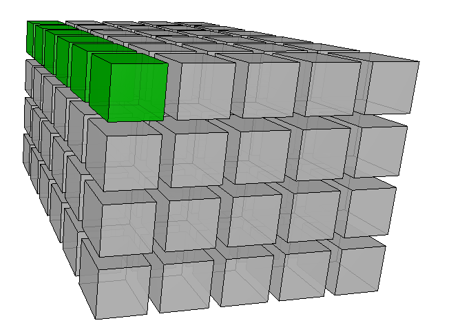
  1. Array instructions within the user program are identified and merged into ‘segments‘.
  2. Segments limits are optimized to hold chunks of suitable workload whose size can be quickly determined at runtime.
  3. Before executing a segment …
    1. The cost of the segment with the current data is computed for each hardware resource.
    2. The best (i.e.: the fastest) hardware resource is selected.
    3. The segments array instructions are optimized for the selected resource and current data.
  4. The kernel is scheduled on the selected resource for asynchronous execution and cached for later reuse.

Likely, this list requires some explanation.

[ Video does not show? Download here: https://ilnumerics.net/media/andere/ILNumerics_Segments_2022.mp4 ]

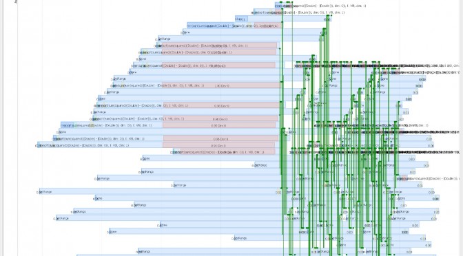
ILNumerics Accelerator takes a new approach to efficient array code execution. Instead of attempting global analysis (the top-down approach which failed in so many projects) we optimize the program from the bottom-up. Our compiler recognizes all fundamental array instructions and expressions thereof, merges them into ‘islands’ (segments) of well-known semantics and execution cost. Each segment contains a small JIT compiler, specialized to quickly compile the segments instructions at runtime into highly optimized low-level codes – for the .NET CLR and for any OpenCL device! This step recognizes and adopts to all hardware and data properties found at runtime. And it maintains compatibility with all .NET platforms.

Currently, we support unary, binary and reduction array instructions provided by ILNumerics Computing Engine and all expressions made thereof. No changes or annotations are required to existing codes. The ILNumerics language supports all features of the Matlab and numpy languages. It will be possible to build connectors to other languages and to custom array libraries exposing similar semantics.

During build each array expression is automatically replaced from the user code files with a call to a specialized, auto-generated segment. Next to hosting a JIT for the array instructions a segment also ‘knows’ the workload of its inherent computations. When at runtime the segment is called, it uses this info to compute the cost for executing the segment on each device and to identify the device suggesting earliest completion. Afterwards, it enqueues the optimized kernel to this device for computation.

It then – without waiting for a result – immediately passes on control to the next segment in the algorithm. Now, if subsequent segments do not depend on each other they are scheduled onto different threads or devices and execute in parallel!

All technical details of the new method are found in the patents and patent applications listed at the end of this article.

Advantages

ILNumerics Accelerator automatically executes your algorithm in the fastest possible way:

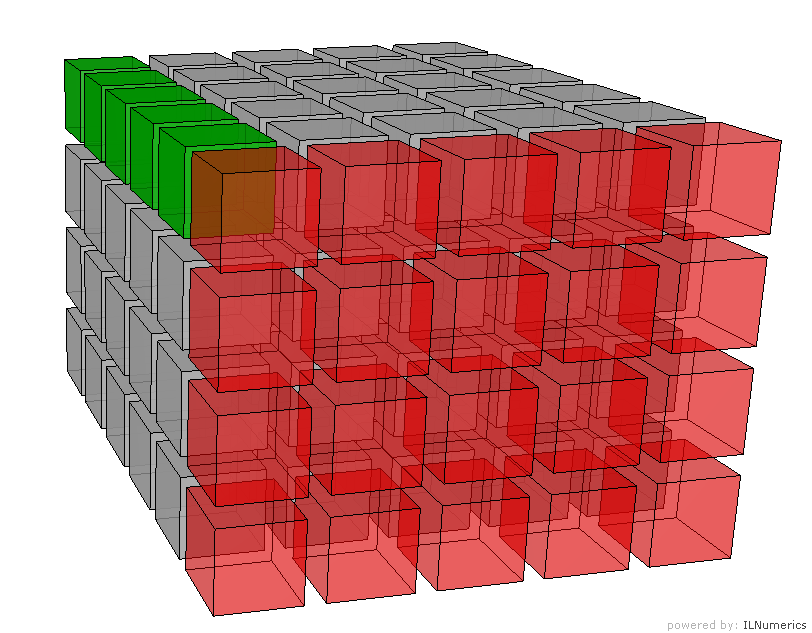
  • During execution it finds chunks of workload which can be computed concurrently.
  • It identifies the best suited hardware device available at this time.
  • For each segment it adopts the execution strategy to the fastest device, and
  • Computes the workload of many segments in parallel.

Therefore, it scales execution times with the hardware without recompilation or manual code adjustments.

Our compiler …

  • Supports vector registers, multiple CPU cores, and all OpenCL devices.
  • Removes temporary arrays and manages memory between devices transparently.
  • Applies many new and important optimizations, on kernel and on segment level.
  • Fully managed solution: it targets the .NET CLR, thus is compatible with all .NET platforms.

… which brings many benefits:

  • Efficient use of all compute resources.
  • No expert effort required.
  • Shorter time to market.
  • Adjusts to new hardware.
  • Maintains maintainability.

“How much faster is it”?

This is a very popular question! A comprehensive answer deserves its own article, really.

In short: it depends on your hardware. It depends on your algorithm. And it depends on your data! The question should rather be: how much more efficiently will it utilize my hardware? For the majority of real-world algorithms is true: as efficient as possible! Moreover, it does so automatically!

(If you are still longing for a number: on 2015-ish hardware we see speed increase rates between 3 and more than 300. Most of the time optimized code runs faster by at least a magnitude.)

Where can I get it ?

ILNumerics Accelerator has entered the public beta phase. It will be released with ILNumerics Ultimate VS version 7. The pre-release is available on nuget. Start here ! General documentation on the new Accelerator is found here. It will subsequently be completed within the next weeks.

Patents

ILNumerics software is protected by international patents and patent applications. WO2018197695A1, US11144348B2, JP2020518881A, EP3443458A1, DE102017109239A1, CN110383247A, DE102011119404.9, EP22156804. ILNumerics is a registered trademark of ILNumerics GmbH, Berlin, Germany.

ILNumerics Accelerator – A better Approach to faster Array Codes, Part I

A Truth most Programmers won’t tell.

TLDR: It was twenty years ago when computer manufacturers, while trying to boost CPU performance, were confronted with the hard wall imposed by physical limitations. It took a long time for everyone involved to realize that individual processors could no longer become significantly faster in the future. The previous approach made it too simple to deal with the constantly growing demands caused by ever larger data and ever more complex programs. Haymo Kutschbach, founder and CEO of ILNumerics explains the challenges involved for automatic parallelization on today’s hardware and why traditional compilers will not satisfy the strong demand for a feasible solution. A better, working approach is presented.

Reading time: 10 minutes

For many decades, the rule applied: “Your program is too slow? Simply buy the latest hardware!” This was made possible by the availability of (general purpose) programming languages, as well as a stream of innovations in processor architectures and the associated compilers. They allowed the programs to be written largely independently of the execution hardware. The compiler adapted abstract codes to the low-level features of the processors. Everything fit together so conveniently!

And then nature threw a spanner in the works on this easy calculation. We’ve seen new computers continueing to obey Moore’s Law and become more powerful with each generation. But this new computing power is now distributed over many processors! A program can only use the new speed if it can use all processors at the same time. In addition, a significant part of the computing power of today’s computers is found in heterogeneous architectures such as GPUs and other accelerator hardware.

The consequences can be observed today in probably every development department: Programs are written abstractly. Efforts are made to create ‘clean code’ that can be tested and maintained. Unfortunately, it is often executed too slowly, though! So you start to examine the codes for optimization potential. You identify individual bottlenecks, decide manually on a parallelization strategy, implement, test and measure again. Many programmers don’t see this as a problem – their expert knowledge guarantees them a good income for many years to come! Since there are no alternatives, the enormous delays in time to market are accepted. Just like the fact that the next generation of devices will again require a complete rewrite for large parts of the software.

Hardware today is far more diverse and heterogeneous than it was 20 years ago. But why is that actually a problem? Why are we still not able to automatically adapt and run our programs on such hardware again?

If it’s too slow, blame the Compiler!

For one, it’s because the compiler market has traditionally been dominated by processor manufacturers. Their compilers served to make their own hardware more accessible. Even though we’ve seen a recent trend towards vendor-independent compilers, they still continue the traditional approach: compiling (“lowering”) code of a general purpose programming language (like C or Fortran) to hardware instructions that can be executed on a specific (and previously selected) processor architecture. What we actually need, however, is a compiler that translates an abstract program for a “computer” – with all its diverse computing resources.

This task, however, is much more demanding! Why? Here we come to the second reason that has so far prevented a working solution: granularity. In order to be able to use parallel resources, the software must contain additional instructions that take care of the distribution of the individual program parts. This additional overhead makes a certain minimum program size (workload) mandatory. Parallelization only makes sense if the gain in speed through parallel execution exceeds the additional management effort!

Here, the term “granularity” refers to the number of individual low -level instructions that a piece of code requires to calculate its result. Apparently, the granularity increases with the size or complexity of a program part, because more low-level instructions are executed at the end. So, in order to make efficient use of parallelism, it is not enough to consider individual instructions of a program. Rather, a compiler must merge larger program parts (‘grains’) and distribute them to the available computing resources . One of the most important challenges of a parallelizing compiler is to find the optimal size of these “chunks” – and thus the optimal granularity.

This brings us to the third reason: complexity. In general, programs can become arbitrarily complex. Compilers have the task of translating programs into another, useful form. But how does one translate information that can be arbitrarily complex? Traditional compilers achieve this goal by limiting their consideration to individual instructions in the program. They know the (manageable) set of possible translations for each of these instructions. The finished program is then little more than the chain of such individual translations. Nevertheless, traditional compilers are already considered to be extremely complex software!

Unfortunately, this “complexity reduction” trick is in direct contradiction to the necessary, minimal granularity described above. A parallelizing compiler must face the challenge of finding an optimal translation even for program chunks that consist of multiple or many instructions. As always, low hanging fruits exist (see e.g.: tensorflow). However, an optimal solution must not restrict itself to individual, specific instructions just because their translation is particularly simple and therefore easy to implement!

And then there is a fourth aspect that also plays into the area of complexity. In addition to the optimal chunk size (granularity), it is also important to identify those grains of a program that can be executed independently of one another. The program analysis required must also take into account the best possible granularity. A compiler must therefore be able to understand large program sections, form chunks of an optimal grain size and execute them efficiently in parallel on heterogeneous hardware.

Ultimately, it is the complexity of this task that has so far prevented such a compiler from being born. In general, development departments still follow the manual approach described earlier. It requires expert knowledge and enormous effort to manually perform the necessary steps (granularity and independence analysis, parallel implementation) for a special program . But despite the enormous amount of time, despite the enormous maintenance issues associated, this approach allows to scratch the surface only! It can neither address nor solve the real problem.

Are we lost?

Not yet! Let’s wrap it up:

  • Traditional compilers work at too low a level of granularity. They consider too few instructions to cover a workload, suitable for efficient parallelization.
  • Previous attempts to include large/all program parts in an analysis have only been successful in a few special cases. Global analysis for general programs is an unsolved problem and, in the opinion of the author, will remain so for a long time to come.

But now we come to the topic of our headline! For a not too small class of programs ILNumerics succeeded in developing a compiler that fulfills all optimality requirements. It is the class of numeric, array-based programs. They are written by scientists, mathematicians, and engineers to encode the innovations of our modern times. They form the core of big data, machine learning and artificial intelligence, and all codes, making use of them. Numerical algorithms realize innovations – moreover: they are these innovations! They allow to formulate great complexity without great effort. They handle huge data and, therefore, require greatest speed.

A development department, faced with the challenge of accelerating its numerical array codes can only select and use the best possible language and libraries there are. Technical requirements often rule out prototyping languages, like numpy and Matlab. Individual parts may be outsourced to GPUs. Other parts are parallelized using multithreading. All of this slows down the industrial development process significantly. It is like writing GUI programs in assembler…

A Better Approach to faster Array Codes

ILNumerics proposes a new, faster approach to the execution of array codes. ILNumerics Accelerator, automatically finds parallel potential in array-based algorithms (as: numpy, Matlab, ILNumerics) and efficiently distributes its workload to heterogeneous computing resources – dynamically and at runtime, when all important information is available. It again scales your algorithm speed to any heterogeneous hardware without recompilation.

The online documentation describes technical details of the ILNumerics Accelerator Compiler. Make sure to register for our newsletter here and don’t miss any news!

Where can I get it ?

ILNumerics Accelerator has entered the public beta phase. It will be released with ILNumerics Ultimate VS version 7. The pre-release is available on nuget. Start here ! General documentation on the new Accelerator is found here. It will subsequently be completed within the next weeks. Read the getting started guide(s), get your hands dirty and please, let us know what you think!

Patents

ILNumerics software is protected by international patents and patent applications. WO2018197695A1, US11144348B2, JP2020518881A, EP3443458A1, DE102017109239A1, CN110383247A, DE102011119404.9, EP22156804. ILNumerics is a registered trademark of ILNumerics GmbH, Berlin, Germany.

Why MINT-students should learn C# instead of Matlab and R

For students who want to prototype and code, there’s a wide range of domain specific programming languages around: R or Matlab – just to name a few – make it quite easy to design new algorithms, analyze data and to plot complex functions. However, bringing innovation from science to enterprise-ready software applications still costs lots of effort, manpower and experience.

Microsoft’s C# has the potential to fully close this gap: in combination with the ILNumerics numerical library, it becomes the perfect environment both for prototyping and creating powerful software. But why is it that the mainstream in science still doesn’t make use of the power of C#, .NET and Visual studio? Well, let’s have a closer look at computing in academia.

Scientific Computing vs. Real-Life Applications

Like in many other areas in academia, the main reason for sticking to out-of-date techniques is “tradition”. That’s why in 2020 there is still a huge gap between mathematical prototyping and industrial-grade production software. Scientists often aim at creating an algorithm solely in order to validate a new model or theory. Once done, they produce a couple of nice looking plots, publish a paper or two and: bye bye.

Unless… there is a greater use to it!

Turning Prototypes into Products

If a model created in science has the potential to earn serious money,  the algorithm created by a mathematician, physicist or microbiologist has to be transformed into something ‘production ready’ that can be used in real life.

This is where many development teams in the biggest enterprises are stuck today: Everytime they want to adapt innovation from science for their own software applications, they have to translate Matlab, numpy or R codes into a modern, managed SW framework. This transformation is where the pain starts: It has to be done! And not only once, but with each update. This causes a whole lot of redundant and boilerplate code – each and every time. This work is expensive: It requires expert knowledge, extensive testing and additional maintenance. And it significantly delays the time to market!

C# + ILNumerics: Perfect Match for High Performance Applications

This pain needs to stop. And this is where modern general purpose languages come into play. C# for example fulfills all the requirements for the design of numerical algorithms! Developer tools such as Visual Studio – especially if complemented with the ILNumerics Array Visualizer und its highly efficient n-dimensional arrays – allow scientists and software developers to design and prototype their algorithms by directly using production-ready tools.

That means: the painful and time consuming transformation from domain specific prototyping code to an industrial software product is no longer necessary, which allows for huge time savings – often more than 50 percent!

Maths, Physics, Engineering: Boost Innovation now!

However, most established scientists in academia today still stick to Matlab, numpy and R – even though it’s not necessary anymore. But fortunately, a new generation of scientists has started to push innovation at universities ahead. They are often familiar with modern programming languages like C#, and they want to use their knowledge to combine academic prototyping with state of the art software development. This new generation will modernize the intersections between science and industry. Their skills will allow companies all over the world to realize all their innovative potential in a much shorter period of time.

That’s why we think any science and engineering student should get familiar with modern programming languages as early as possible: It will help him or her to boost innovation in their field all over the world!

N-dim Array Broadcasting Efficiency in ILNumerics 4.10

Next to other great improvements in version 4.10 of ILNumerics Ultimate VS, it is especially one new feature which requires some attention: general broadcasting for n-dimensional ILArrays.

Broadcasting as a concept today is found in many popular mathematical prototyping systems. The most direct correspondence probably exists in the numpy package. Matlab and Octave offer similar functionality by means of the bsxfun function.

The term ‘broadcasting’ refers to a binary operator which is able to apply an elementwise operation to the elements of two n-dimensional arrays. The ‘operation’ is often as simple as a straight addition (ILMath.add, ILMath.divide, a.s.o.). However, what is special about broadcasting is that it allows the operation even for the case where both arrays involved do not have the same number of elements.

Broadcasting in ILNumerics prior Version 4.10

In ILNumerics, broadcasting is available for long already. But prior version 4.10 it was limited to scalars operating on n-dim arrays and vectors operating on matrices. Therefore, we had used the term ‘vector expansion’ instead of broadcasting. Obviously, broadcasting can be seen as a generalization of vector expansion.

Let’s visualize the concept by considering the following matrix A:

A

1  5   9  13  17
2  6  10  14  18
3  7  11  15  19
4  8  12  16  20

Matrix A might represent 5 data points of a 4 dimensional dataset as columns. One common requirement is to apply a certain operation to all datapoints in a similar way. In order to, let’s say, scale/weight the components of each dimension by a certain factor, one would multiply each datapoint with a vector of length 4.


ILArray<double> V = new[] { 0.5, 3.0, 0.5, 1.0 };

0.5
3.0
0.5
1.0

The traditional way of implementing this operation would be to expand the scaling vector by replicating it from a single column to a matrix matching the size of A.

VExp = repmat(V, 1, 5); 

0.5  0.5  0.5  0.5  0.5
3.0  3.0  3.0  3.0  3.0
0.5  0.5  0.5  0.5  0.5
1.0  1.0  1.0  1.0  1.0

Afterwards, the result can be operated with A elementwise in the common way.

ILArray<double> Result = VExp * A;

0.5   2.5   4.5   6.5   8.5
6.0  18.0  30.0  42.0  54.0
1.5   3.5   5.5   7.5   9.5
4.0   8.0  12.0  16.0  20.0

The problem with the above approach is that the vector data need to be expanded first. There is little advantage in doing so: a lot of new memory is being used up in order to store completely redundant data. We all know that memory is the biggest bottleneck today. We should prevent from lots of memory allocations whenever possible. This is where vector expansion comes into play. In ILNumerics, for long, one can prevent from the additional replication step and operate the vector on the matrix directly. Internally, the operation is implemented in a very efficient way, without replicating any data, without allocating new memory.

ILArray<double> Result = V * A;

0.5   2.5   4.5   6.5   8.5
6.0  18.0  30.0  42.0  54.0
1.5   3.5   5.5   7.5   9.5
4.0   8.0  12.0  16.0  20.0

Generalizing for n-Dimensions

Representing data as matrices is very popular in scientific computing. However, if the data are stored into arrays of other shapes, having more than two dimensions, one had to fall back to repmatting in order for the binary operation to succeed. This nuissance has been removed in version 4.10.

Now it is possible to apply broadcasting to two arrays of any matching shape – without the need for using repmat. In order for two arrays to ‘match‘ in the binary operation, the following rules must be fullfilled:

  1. All corresponding dimensions of both arrays must match.
  2. In order for two  corresponding dimensions to match,
    • both dimensions must be of the same length, or
    • one of the dimensions must be of length 1.

An example of two matching arrays would be a vector running along the 3rd dimension and a 3 dimensional array:

3D Cubes 4 Broadcasting2In the above image the vector (green) has the same length as the corresponding dimension of the 3D array (gray). The size of the vector is [1 x 1 x 6]. The size of the 3D array is [4 x 5 x 6]. Hence, any dimension of both, the vector and the 3D array ‘match’ in terms of broadcasting. A broadcasting operation for both, the vector and the array would give the same result as if the vector would be replicated along the 1st and the 2nd dimensions. The first element will serve all elements in the first 4 x 5 slice in the 1-2 plane. This slice is marked red in the next image: 3D Cubes 4 Broadcasting_sliceNote that all red elements here derive from the same value – from the first element of the green vector.  The same is true for all other vector elements: they fill corresponding slices on the 3D array along the 3rd dimension.

Slowly, a huge performance advantage of broadcasting becomes clear: the amount of memory saved explodes when more, longer dimensions are involved.

 Special Case: Broadcasting on Vectors

In the most general case and if broadcasting is blindly applied, the following special case potentially causes issues. Consider two vectors, one row vector and one column vector being provided as input parameters to a binary operation. In ILNumerics, every array carries at least two dimensions. A column vector of length 4 is considered an array of size [4 x 1]. A row vector of length 5 is considered an array of size [1 x 5]. In fact, any two vectors match according to the general  broadcasting rules.

As a consequence operating a row vector [1 x 5] with a column vector [4 x 1] results in a matrix [4 x 5]. The row vector is getting ‘replicated’ (again, without really executing the replication) four times along the 1st dimension, and the column vector 5 times along the rows.

array(new[] {1.0,2.0,3.0,4.0,5.0}, 1, 5) +array(new[] {1.0,2.0,3.0,4.0}, 4, 1)

<Double> [4,5]
[0]:          2          3          4          5          6
[1]:          3          4          5          6          7
[2]:          4          5          6          7          8
[3]:          5          6          7          8          9

Note, in order for the above code example to work, one needs to apply a certain switch:

Settings.BroadcastCompatibilityMode = false;

The reason is that in the traditional version of ILNumerics (just like in Matlab and Octave) the above code would simply not execute but throw an exception instead. Originally, binary operations on vectors would ignore the fact that vectors are matrices and only take the length of the vectors into account, operating on the corresponding elements if the length of both vectors do match. Now, in order to keep compatibility for existing applications, we kept the former behavior.

The new switch ‘Settings.BroadcastCompatibilityMode’ by default is set to ‘true’. This will cause the Computing Engine to throw an exception when two vectors of inequal length are provided to binary operators. Applying vectors of the same length (regardless of their orientation) will result in a vector of the same length.

If the ‘Settings.BroadcastCompatibilityMode’ switch is set to ‘false’ then general broadcasting is applied in all cases according to the above rules – even on vectors. For the earlier vector example this leads to the resulting matrix as shown above: operating a row on a column vector expands both vectors and gives a matrix of corresponding size.

Further reading: binary operators, online documentation

ILNumerics for Scientists – Going 3D

Recap

Last time I started with one of the easiest problems in quantum mechanics: the particle in a box. This time I’ll add 1 dimension and we’ll see a particle in a 2D box. To visualize its wave function and density we need 3D surface plots.

2D Box

This time we have a particle that is confined in a 2D box. The potential within the box is zero and outside the box infinity. Again the solution is well-known and can be found on Wikipedia. This time the state of the wave function is determined by two numbers. These are typically called quantum numbers and refer to the X and the Y direction, respectively.

The absolute size of the box doesn’t really matter and we didn’t worry about it in the 1D case. However, the relative size of the length and the width make a difference. The solution to our problem reads

$\Psi_{n,k}(x,y) = \sqrt{\frac{4}{L_x L_y}} \cdot \sin(n \cdot \pi \cdot x / L_x) \cdot \sin(k \cdot \pi \cdot y / L_y)$

The Math

Very similar to the 1D case I quickly coded the wave function and the density for further plotting. I had to make sure that the arrays are fit for 3D plotting, so the code looks a little bit different compared to last post’s

     public static ILArray<double> CalcWF(int EVXID, int EVYID, double LX, double LY, int MeshSize)
     {
        ILArray<double> X = linspace<double>(0, LX, MeshSize);
        ILArray<double> Y = linspace<double>(0, LY, MeshSize);

        ILArray<double> Y2d = 1;
        ILArray<double> X2d = meshgrid(X, Y, Y2d);

        ILArray<double> Z = sqrt(4.0 / LX / LY) * sin(EVXID * pi * X2d / LX) * sin(EVYID * pi * Y2d / LY);

        return Z.Concat(X2d,2).Concat(Y2d,2);
     }

Again, this took me like 10 minutes and I was done.

The Visualization

This time the user can choose the quantum numbers for X and Y direction, the ratio between the length and the width of the box and also the number of mesh points along each axis for plotting. This makes the visualization panel a little bit more involved. Nevertheless, it’s still rather simple and easy to use. This time it took me only 45 minutes – I guess I learned a lot from last time.

The result

Here is the result of my little program. You can click and play with it. If you’re interested, you can download the Particle2DBox source code. Have fun!

Particle2DBoxThis is a screenshot of the application. I chose the second quantum number along the x axis and the fourth quantum number along the y axis. The box is twice as long in y direction as it is in x direction. The mesh size is 100 in each direction. On the left hand side you see the wave function and on the right hand side the probability density.

Directions to the ILNumerics Optimization Toolbox

As of yesterday the ILNumerics Optimization Toolbox is out and online! It’s been quite a challenge to bring everything together: some of the best algorithms, the convenience you as a user of ILNumerics expect and deserve, and the high performance requirements ILNumerics sets the scale on for. We believe that all these goals could be achieved quite greatly.

Continue reading Directions to the ILNumerics Optimization Toolbox

ILNumerics for Scientists – An easy start

Motivation

I’ve been working as a scientist at universities for 10 years before deciding to go into industry. The one thing I hated most was coding. At the end of the day coding for scientists is like running for a football player. Obviously, you need it but it’s not what you’re here for.

I really dreaded the coding and the debugging. So much precious time for something that was so clear on paper and I just wanted the solution of my equations to see whether my idea made sense or not. More often than not scientists find that their idea was not so great and now they had spent so much time coding just to find out that the idea didn’t work. Continue reading ILNumerics for Scientists – An easy start

C# for 3D visualizations and Plotting in .NET

2D and 3D Visualizations are an important feature for a wide range of domains: both software developers and scientists often need convenient visualization facilities to create interactive scenes and to make data visible. The ILNumerics math library brings powerful visualization features to C# and .NET: ILView, the ILNumerics Scene Graph API and its plotting engine. We’d like to give an overview over our latest achievements.

ILView: a simple way to create interactive 3d visualizations

We have created ILView as an extension to our interactive web component: It allows you to simply try out ILNumerics’ 2d and 3d visualization features by chosing the output format .exe in our visualization examples. But that’s not all: ILView is also a general REPL for the evaluation of computational expressions using C# language. ILView is Open Source – find it on GitHub!

Screenshot of ILView
Using ILView for interactive 3D Visualization

ILNumerics Scene Graph: realize complex visualizations in .NET

The ILNumeric’s scene graph is the core of ILNumerics’ visualization engine. No matter if you want to create complex interactive 3D visualizations, or if you aim at enhancing and re-configuring existing scenes in .NET: The ILNumerics scene graph offers a convenient way to realize stunning graphics with C#. It uses OpenGL, GDI, and it’s possible to export scenes into vector and pixel graphics.

Screenshot of an interactive 3D scene
Using C# for 3D visualizations: the ILNumerics Scene Graph

Scientific Plotting: visualize your data using C#

With ILNumerics’ visualization capabilities, C# becomes the language of choice for scientists, engineers and developers who need to visualize data: Our plotting API and different kinds of plotting types (contour plots, surface plots etc.) make easy work of creating beautiful scientific visualizations.

Screenshot of a Surface Plot in ILNumerics
Scientific Plotting in .NET: A Surface Plot created with ILNumerics