Overview
Testing Visual Studio extensions against different versions of Visual Studio poses many challenges due to the large array of Visual Studio versions. The following post describes a generally applicable solution on the basis of the example of the ILNumerics Array Visualizer extension. Furthermore, this article will elaborate on how we managed to perform (relatively) stable test integrations into our build scripts.
When implementing new features into your code, today it is a well accepted fact that your code needs to be tested against as much potential scenarios as possible. You need to write unit tests and integration tests to anticipate the behavior of your application and to ensure it is working in the expected way in all possible situations.
So how do you test a Visual Studio extension? First of all, you should define integration test scenarios, to check if your code works as expected. Make sure to include many different scenarios to achieve maximum code coverage.
What do we have to test?
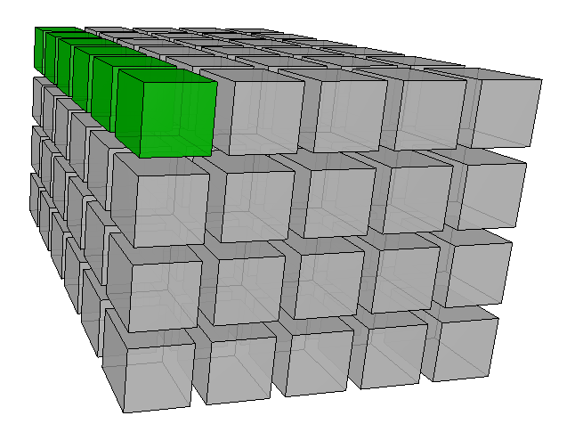
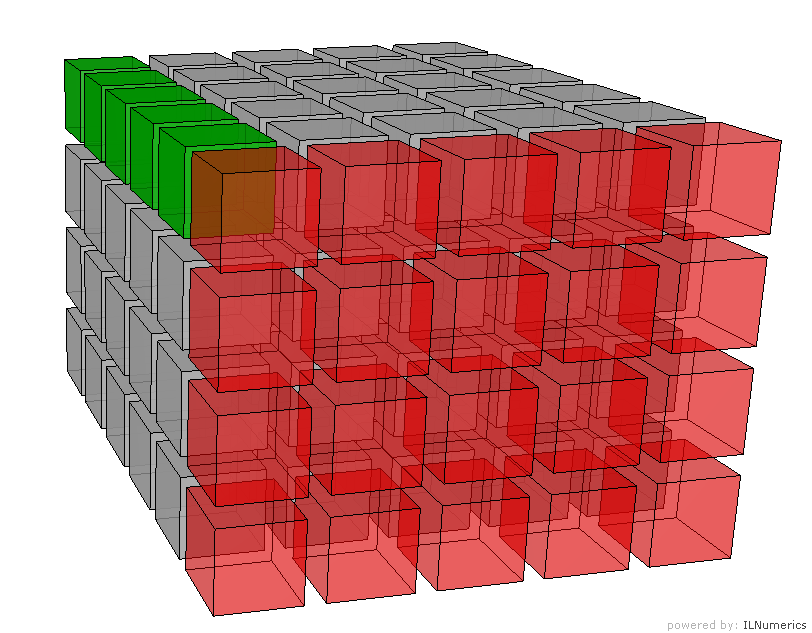
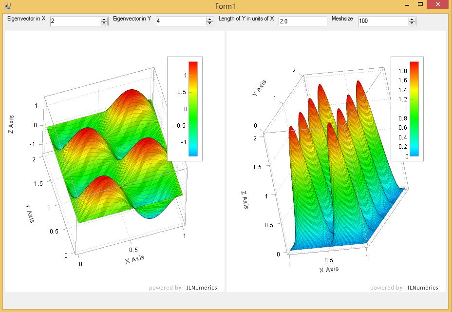
The ILArrayVisualizer is a Visual Studio extension that allows you to visualize large data sets in a number of ways during your debug session. Our current version 4.11 can not only be installed in different versions of Visual Studio but also supports various project languages and data types. To be precise, the full parameter space has the following dimensions:
- Visual Studio versions: 2010, 2012, 2013, 2015
- Programming languages: C#, Visual Basic, F#, Fortran, C/C++
- All common project types: dll, exe
- Platforms: 32/ 64 bit
- All supported array types for each individual language: 1D/ n-dim, ILArray<T>, pointers, std::array, a.s.f.
- All numeric element types: double, float, (f)complex, (u)int32/16/64), bytes, char, …
- Arrays may also contain special numbers (NaNs, Inf), empty shapes in various forms, uninitialized arrays, or NULL.
The huge parameter space forbids any test strategies that are based on manually performed testing. In order to cover the most important cases only, we’ve identified more than 1000 integration test cases! As a result, automated integration tests are obligatory. Furthermore, the tests need to be integrated into our build system and have to support manual (debug) as well as automated (release) triggers.
One may ask: why not simply testing the array visualizer service in a regular unit test project? Why do we need to perform integration tests inside Visual Studio at all? The answer is that Visual Studio provides a complex environment which needs to fullfill a huge amount of requirements and to support us in a vast number of situations. A complex interaction with the Visual Studio debugger uncovers incompatibilities here and there. Performing automated integration tests over nearly the whole parameter space provides good coverage of all expected usage scenarios and indeed allowed us to identify any incompatibilities – and to work around them.
First: Define a Testing Strategy, Second: Write the Code
To test the ILArrayVisualizer, we had to define a testing strategy first. The testing strategy includes procedures that are performed during each test run and therefore have to be automated in a reliable way:
- Run the experimental instance of Visual Studio including the installed ILArrayVisualizer extension.
- Load a predefine test project of a certain programming language as supported by the Array Visualizer.
- Stop the debugger at a certain, predefined position in the project.
- Inspect various array instances and check that the Array Visualizer service is able to deliver correct results for it.
Hereby, the main challenge was that integration tests for Visual Studio extensions must run inside another instance of Visual Studio and that we needed a method to ensure this reliably for all supported version of Visual Studio. The test target (our extension project) must be installed in the target Visual Studio version in advance. Consequently, the tests were run in a semi-automatic mode: Our testing framework had to be executed once for each Visual Studio version.
How to Run the Test Code in an Experimental Instance of Visual Studio
Do you know how to write standard unit tests in C#? It is quite simple: While the attribute [TestClass] is applied to each test class object, the attribute [TestMethod] is applied to each test method. You can find more information about all attributes in the official MSDN Article “Anatomy of Unit Tests”.
For the integration tests things become a little more demanding. Let’s take a look at our testing strategy one more time: For each test method we have to create a new experimental instance of Visual Studio. Since we have to run more than 1000 test cases for each Visual Studio version, creating new instances, opening the test project and other actions will take too much time. So let’s change our strategy: We will start the experimental instance only once for all test methods, leveraging the attributes mentioned above.
To begin with, we implemented a [ClassInitialize] method, which runs the experimental instance for our test methods once:
[ClassInitialize]
[HostType("VS IDE")]
[TestProperty("VsHiveName", "14.0Exp")]

public static void TestClassInitialize(TestContext testContext)
{
// test class initialize
}
- The attribute [ClassInitialize] tells the compiler that the following public method is defined as a constructor for our test class.
- The attribute [HostType(“VS IDE”)] defines that the following method should be executed in Visual Studio IDE. It’s also possible to create an instance of another host type. You can read more about it in MSDN.
- The attribute [TestProperty(“VsHiveName”,”14.0Exp”)] defines that the following test method will be executed in Visual Studio Version 14.0(VS 2015) inside the experimental instance.
Why do we actually need an Experimental instance? Because it gives us a way to run, debug and test our extension code – from inside Visual Studio. The Experimental instance runs parallel to the
‘main’ instance. It allows a clear separation in terms of configuration and installed extensions. During the development of our extension, we can build and run our project by installing the target VSIX extension only inside the experimental instance.
Experimental Instance is launched, what’s next?
As our test method runs in an experimental instance of Visual Studio, we need to obtain an environment DTE. The DTE object is the root of the automation model, which other object models often call “Application”.
ILArrayVisualizer Extension works in the COM model of Visual Studio and as such has its own GUID which is used to identify the service among the list of available serives in Visual Studio. To call the methods to be tested, we also need to obtain a service provider. By using the service provider, we can access the ILArrayVisualizer Service inside the experimental instance and call the methods to be tested.
var m_envdte = VsIdeTestHostContext.Dte;
var m_shellservice = VsIdeTestHostContext.ServiceProvider.GetService(typeof(SVsShell)) as IVsShell;

Guid packageGuid = new Guid("XXXXXXX-XXXX-XXXX-XXXX-XXXXXXXXXXXX");

m_shellservice.LoadPackage(ref packageGuid, out m_package);

m_serviceProvider = new ServiceProvider(m_envdte as Microsoft.VisualStudio.OLE.Interop. IServiceProvider);
What about the Debugger and the test methods?
To obtain a debugger session descriptor in another instance of Visual Studio, the IDE uses the following code:
var m_debugger = m_envdte.Debugger;
So, this refers to the Debugger object inside the (experimental) instance referenced by the Environment DTE object. This way it is actually possible to control other instances of the VS IDE.
Basically, each integration test simulates the actions a regular user of the Array Visualizer would take: inside a debug session she inspects certain arrays (large variation here!) in the Array Visualizer and receives a number of correct outputs for them. All test projects (i.e. the debug target handled by our virtual users) have to be predefined. Each language comes with its own test projects files, in which we defined a large set of supported array expressions, including a reasonable number of edge cases. The projects are loaded via remote control from our integration tests, are started and halted in debug mode inside the remotely controlled Visual Studio instance. Visual Studio is used to set breakpoints in them, to stop the debugger and perform queries to the Array Visualizer service – one query for each of the predefined test array objects (more than 1000 test arrays exist).
In our case, we just open one of the predefined C++, C#, Visual Basic or FORTRAN project, run it in a new debug session, and iterate all contained array expressions by calling the evaluate() method of our ILArrayVisualizer service on it – all from our testing framework.
To open the existing projects and add those, we use the following method:
EnvDTE.Solution.AddFromFile(FileName);
To build the Solution:
EnvDTE.Solution.SolutionBuild.Build(true);
// True means, wait until build is ready.
As we get debugger session descriptor, setting the breakpoint is as easy as:
Debugger.Breakpoints.Add(FileName, LineNumber);
All necessary initialization code could be packed into the test class initializer. In this case only one experimental instance will be created for each language and platform and reused to test many test methods at once.
Passing the Test Code to Visual Studio IDE Experimental Instance
By default, all integration tests are hosted and run in the VSTestHost.exe process. To pass the test code to be executed to the experimental instance (in another environment), we have to use the Test Host Adapter. UIThreadInvoker allows us to implement a delegate method and pass it to our test environment.
UIThreadInvoker.Initialize();
UIThreadInvoker.Invoke((ThreadInvoker)delegate ()
{
// some test cases
}
The integration tests are not only for finding bugs inside your code, but also help you write correct code. To write unit tests, we specified how a class or method should work first. Read more about it here: “Test-Driven Development”. We used this strategy to write a correct expression evaluator for C++ code for the ILArrayVisualizer. We wrote all possible test methods for each possible expression and tested the expected values – for all supported languages.
When implementing a new feature it is crucial to develop a testing strategy to ensure proper functionality and achieve maximum code coverage. In Visual Studio there are testing tools that you can use for this purpose.